This tutorial walks you through how to use linear regression to predict customer spending based on activity data from an ecommerce platform. It's written step-by-step to help you learn both the coding and the reasoning behind each action.
About the Dataset
This dataset contains information about customers who shop for clothing online. The store offers in-person style consultations, and customers often continue their shopping experience digitally—either on a mobile app or through the website.
The purpose of the dataset is to help the company understand where to focus its user experience efforts: should it invest more in improving the mobile app or the website? The dataset includes various metrics such as average session length, time spent on app vs website, membership duration, and total yearly spending.
Sample of the Dataset
Below is a preview of the ecommerce dataset. It includes customer contact info (which we later drop), user activity metrics, and their total yearly spending:
| Avg. Session Length | Time on App | Time on Website | Length of Membership | Yearly Amount Spent | |
|---|---|---|---|---|---|
| mstephenson@fernandez.com | 34.50 | 12.66 | 39.58 | 4.08 | $587.95 |
| hduke@hotmail.com | 31.93 | 11.11 | 37.27 | 2.66 | $392.20 |
| pallen@yahoo.com | 33.00 | 11.33 | 37.11 | 4.10 | $487.55 |
| riverarebecca@gmail.com | 34.31 | 13.72 | 36.72 | 3.12 | $581.85 |
The original dataset is available on Kaggle.
1. Load and Clean the Data
We begin by loading the dataset and cleaning the column names. Some fields, such as Address, contain line breaks and are enclosed in quotation marks, which is important to handle correctly when reading the file.
import pandas as pd

# Load the dataset using the correct file extension and quoting
df = pd.read_csv('dataset.csv', quotechar='"')

# Replace spaces with underscores for easier access in Python
df.columns = [col.strip().replace(" ", "_") for col in df.columns]

# Print all column names to inspect the structure
print(df.columns)
Output:
Index(['Email', 'Address', 'Avatar', 'Avg._Session_Length', 'Time_on_App',
       'Time_on_Website', 'Length_of_Membership', 'Yearly_Amount_Spent'],
      dtype='object')
Explanation: We cleaned column names to avoid problems when referencing them in code. Inspecting columns helps understand what features are available for prediction.
Tip: When reading this
.csvfile usingpandas.read_csv(), make sure to includequotechar='"'to correctly handle the quoted multiline address fields.
2. Drop Irrelevant Columns
Some columns like Email, Address, and Avatar are identifiers or not numeric—so they're not helpful for regression.
df = df.drop(['Email', 'Address', 'Avatar'], axis=1)
Explanation: Machine learning models work best with numerical data. These removed fields don't influence a person's spending behavior.
3. Split the Dataset
Next, we separate the data into input features X and the target value y (the thing we want to predict), and split into training and test sets.
from sklearn.model_selection import train_test_split

X = df.drop(['Yearly_Amount_Spent'], axis=1)  # Input features
y = df['Yearly_Amount_Spent']                 # Target variable

X_train, X_test, y_train, y_test = train_test_split(
    X, y, test_size=0.2, random_state=42)
Explanation: We use 80% of the data to train the model, and 20% to test how well it works. This prevents overfitting and gives us a realistic assessment of model performance.
4. Train the Linear Regression Model
Now we create a linear regression model using scikit-learn and train it using our training data.
from sklearn.linear_model import LinearRegression

model = LinearRegression()
model.fit(X_train, y_train)
Explanation: The model learns the best-fitting line through the training data to make predictions on new data. Linear regression finds the optimal coefficients for each feature.
5. Evaluate the Model
We test our model by making predictions and comparing them to actual values using error metrics.
from sklearn.metrics import mean_absolute_error, mean_squared_error, r2_score

y_pred = model.predict(X_test)

print("MAE:", mean_absolute_error(y_test, y_pred))
print("MSE:", mean_squared_error(y_test, y_pred))
print("R² Score:", r2_score(y_test, y_pred))
Model Evaluation Results
MAE: 8.558441885315203
MSE: 109.86374118393957
R² Score: 0.9778130629184127
Explanation:
- MAE (Mean Absolute Error): On average, our predictions are off by about $8.56
- MSE (Mean Squared Error): Squared version of error—penalizes large mistakes more heavily
- R² Score: Shows that 97.78% of the variation in spending is explained by our model (1.0 would be perfect)
6. Visualize the Predictions
We use a scatter plot to compare actual values to predictions. A perfect model would show all points on a straight diagonal line.
import matplotlib.pyplot as plt

plt.scatter(y_test, y_pred)
plt.xlabel("Actual")
plt.ylabel("Predicted")
plt.title("Actual vs. Predicted Yearly Amount Spent")
plt.show()
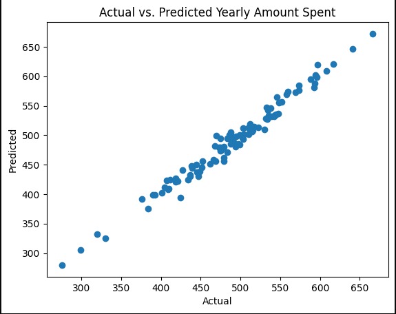
Explanation: This plot helps us visually check the accuracy. The closer the dots are to a 45-degree diagonal line, the better our predictions.
Understanding Feature Importance
Let's examine which features have the most impact on spending predictions:
# Get feature coefficients
feature_names = X.columns
coefficients = model.coef_

# Create a DataFrame for better visualization
feature_importance = pd.DataFrame({
    'Feature': feature_names,
    'Coefficient': coefficients
}).sort_values('Coefficient', key=abs, ascending=False)

print(feature_importance)
This analysis helps the business understand which metrics most strongly correlate with customer spending, informing strategic decisions about where to focus development efforts.
Business Insights
Based on our model results:
- High Accuracy: With an R² score of 0.978, we can confidently use this model for business predictions
- Feature Analysis: The coefficients reveal which customer behaviors drive higher spending
- Strategic Focus: Understanding app vs. website engagement helps prioritize development resources
Next Steps
This foundational example demonstrates key machine learning concepts:
- Data preprocessing and cleaning
- Feature selection and engineering
- Model training and evaluation
- Performance visualization and interpretation
You can now explore more advanced techniques:
- Polynomial regression for non-linear relationships
- Feature engineering to create new predictive variables
- Cross-validation for more robust model evaluation
- Regularization techniques (Ridge, Lasso) to prevent overfitting
Conclusion
Linear regression provides an excellent starting point for predictive modeling in ecommerce. The high accuracy achieved (97.78% R² score) demonstrates that customer engagement metrics are strong predictors of spending behavior.
This approach enables data-driven decision making, helping businesses optimize their digital experiences based on quantifiable customer behavior patterns.
Want to dive deeper into machine learning for business applications? The complete code for this tutorial is available on our GitLab repository. For custom ML solutions for your business, contact our team.